Backpropagating through time

Or, How come BP hasn’t been invented earlier?

In retrospect, the extension to the hidden-layer problem is embarrassingly trivial. I mean, all you have to do is take a threshold logic neuron, as Bernie Widrow did, and just make the slope of that step finite, and then you can solve the whole thing by the gradient descent method using the chain rule of calculus. So, just going from something that has an infinite slope to a finite slope — that's the whole problem. It's so trivial it's embarrassing.

(1993 interview with Jack Cowan, in Talking Nets: An Oral History of Neural Networks )

This post is an attempt to organize some thinking and reading I’ve done around the history of the Backpropagation (BP) algorithm for neural networks, and particularly the question, hinted on in Jack Cowan’s quote above: how come BP hasn’t been invented earlier?

I don’t intend to offer a definitive answer (there probably isn’t any one definitive answer anyways). Instead I will try to highlight a few angles, some of which might be contradicting and some complementing each other. I will try to go back to original sources whenever possible, but hopefully still keep the load of long quotes under control.

It is helpful to isolate the elements of BP, to serve as a guide for the reading. This is because there are in fact several ideas put together, and not all of them necessarily originated in the same time and place. I will use the following list:

• Using an error as a teaching signal

• Propagating errors “backward” from the output unit to upstream units

• Using the gradient of the error (or “loss”) function to determine updates

• Doing all of the above in the context of learning in a “neural network” or some other “adaptive” system

What actually has been invented before

Here this partition into the key elements might help. Each idea on its own, and even some pairwise and triple-wise combinations, predates the actual form of BP as we recognize it today. It’s the combination of all of them together that for some reason took ~25 years or so to get at.

Using an explicit error signal to drive learning (or “adaptation”) has been suggested by many authors. Prominent examples are Rosenblatt’s Perceptron and Widrow and Hoff’s Adaline. It’s worth mentioning that this idea is not the only one possible. For example in the previous post we saw Selfridge’s perspective on how to do supervised learning, without explicitly using example-by-example error, but rather adjusting as to increase some “fitness” overall. There are similar ideas (with actual implementation details) in Mattson 1959 (A Self-Organizing Binary System) under the architecture:

Note that here the feedback to the system is “performance” and not error (again, similar to the idea we saw in Selfridge’s overview).

By contrast, in Widrow and Hopf Adaline (Adaptive Switching Circuits, 1960), the adjusting part is particularly related to the (online) errors made by the system.

Moreover, the Adaline algorithm is a form of online/stochastic gradient descent, relying on the insight that the gradient for the online error (i.e., on a single-example basis) can be computed very easily (we will return to this point later on).

So, Adaline already had 3 out of the 4 concepts of the list we started with. But there’s no propagation of error backwards; the system is a “1-layer”, adaptive linear filter.

The Perceptron is the other well-known architecture of that time, which was basically very similar.¹ In his Principles of Neurodynamics book, Rosenblatt goes a step further to actually discuss the “multi-layered” case:

In the foregoing chapters, we have almost exhausted the possible ramifications of minimal three-layer perceptrons, having an S→A→R topology. Only one constraint remains to be dropped, in order to obtain the most general system of this class: this is the requirement that S to A-unit connections must have fixed values, only the A to R connections being time-dependent. In this chapter, variable S-A connections will be introduced, and the application of an error-correction procedure to these connections will be analyzed.

[…]

The difficulty is that whereas R*, the desired response, is postulated at the outset, the desired state of the A-unit is unknown. We can only say that we desire the A-unit to assume some state in which its activity will aid, rather than hinder, the perceptron in learning the assigned classification or response function.

And he even using the term back-propagation:

The procedure to be described here is called the "back-propagating error correction procedure" since it takes its cue from the error of the R-units, propagating corrections back towards the sensory-end of the network if it fails to make a satisfactory correction quickly at the response end.

However the procedure itself is not gradient learning. It relies on some (inherently) stochastic updates (and while not explained this way, this was possibly introduced to overcome non-differentiability since all the units here are supposedly binary units).

There’s more to say about the discussion of the multi-layered case in Rosenblatt (chapter 13 of Principles of Neurodynamics) but I’ll conclude here by claiming that, similar to Adaline, the Perceptron (in the broad sense of Rosenblatt’s work) also had 3 out of the 4 concepts (for a different 3!), but was missing the recognition of using gradients to propagate the errors backward.

One more issue to talk about is the technicality of actually computing (efficiently) the partial derivatives of some complex “layered” function. Today this is called “reverse-mode automatic differentiation”. As with the rest of the components, this by itself predates the Backpropagation algorithm for neural networks. Seppo Linnainmaa provided what is commonly referred to as the earliest implementation during the early 70’s.² However, Linnainmaa’s work was done in a completely different context (roughly, numerical analysis) without making any connection to adaptive or learning systems. A similar case is that of the earlier works of Paul Werbos, who also developed an algorithm for automatic differentiation in 1974. The context here is closer to “ours”, as Werbos was interested in fitting non-linear statistical models to data. However, making the conceptual connection of this technique to adaptive or learning systems, and to neural networks, would only came later in the early 80’s (around the same time that BP was “invented” all over). To conclude, I would say that these early works on automatic-differentaiton had 2 out of 4 of the elements we started with (but didn’t have the relation to learning/adapting systems).

Some thoughts on “novelty”

This is a good place for a short break to discuss what probably should have been the disclaimer for this post. The one thing I came to appreciate by doing these “historic” readings is how ideas for themselves are almost never “new”. That’s fine, though: scientific work is incremental and always has some context to it, and this context always contain some prior work as well.

So just to be clear, the goal here is not to answer a question like “who invented BP” and assign personal credits (I will leave this sort of discussions to others). I think it’s more interesting and productive to understand what we even mean by “inventing BP” — what were the key components required? where did they originate from? what it took to put all of them together? and what were the conditions that allowed some ideas to finally “stick”, while others were given-up? In that sense, I think the very attribution of “inventing BP” to any particular researcher will always be simplistic, and missing the point(s).

Was it deemed un-important or irrelevant to have “multi-layered” networks?

A potential answer for our original question is: they just didn’t think it was important. But this answer can be very convincingly ruled out. That multi-layered (and non-linear in general) systems will be required and helpful was very much recognized and appreciated from early on. We’ve already seen the intuition about hierarchical processing for “features extraction” and pattern recognition in Selfridge and Dinneen in a previous post. Let’s see some examples.

The early studies on linear classification had well-recognized the limitation of it being linear. For example, in Mattson we find:

By changing the w, values and T, different mapping functions can be obtained. For example, with this device one can obtain 14 different mapping functions for two-input variables, 104 for three-input variables, and approximately 1900 for four-input variables. These different mapping functions are termed "linearly separated" truth functions.

[…]

By interconnecting devices of this type, each one realizing a different linearly separated function, and feeding their outputs into an AND or OR device, any logical function can be obtained. This is easily shown since a single device of this type can realize the AND or OR function of n-variables and any Boolean function can be written as a sum of products or product of sums.

including the (beautiful) figures:

Similar points are being made in Widrow and Hopf:

Linearly separable pure patterns and noisy versions of them are readily classified by the single neuron. Non-linearly separable pure patterns and their noisy equivalents can also be separated by a single neuron, but absolute performance can be improved and the generality of the classification scheme can be greatly increased by using more than one neuron.

And finally, in Rosenblatt, where the argument is perhaps less “technical” but the intuition for the importance of learning a multi-layered network is clearly expressed (as we’ve in fact seen earlier in this post):

It would seem that considerable improvement in performance might be obtained if the values of the S to A connections could somehow be optimized by a learning process, rather than accepting the arbitrary or pre-designed network with which the perceptron starts out. It will be seen that this is indeed the case, provided certain pitfalls in the design of a reinforcement procedure are avoided.

As a side comment, note how this issue of linear separability shows up here way before Minsky and Pappert’s notorious Perceptrons book. I have never fully bought into the explanation of “It’s all Minsky’s fault” on the ‘abandoning’ neural networks. But this post is getting too long as it is, and I will keep a more focused discussion of Perceptrons to another time. Still, while at it, I will let Minsky’s words start the next section.

Hardware, software, and programming

Today, people often speak of neural networks as offering a promise of machines that do not need to be programmed. But speaking of those old machines in such a way stand history on its head, since the concept of programming had barely appeared at that time.

(Minsky and Pappert, Prologue to the 2nd edition of Perceptrons, 1988)

The “old machines” being mentioned here are the adaptive/learning systems of the 1950’s. It’s easy (at least for me) to forget to appreciate that the people developing these algorithms had to build them in hardware.

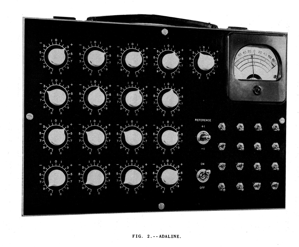
This, of course, is a huge implementation detail. Even the most basic questions of how you physically modify the “weights”, and how you store those weights on the device, are not trivial. For example, in the first versions of Adaline the learning had to be done “by hand”, by actually switching the knobs controlling each weight:

Widrow and Hopf next invented the “Memistor” (Memory Resistor), an electric component that could be automatically controlled to increase/decrease its resistance (by plating more or removing graphite) which allowed the learning to be done automatically by just providing the target signal.³ Just have a loog at this brilliant video of Widrow himself demonstrating both versions of Adaline to students (I’m unfortuntately not sure what year this was recorded in):

So here’s an entertaining idea. If you were to built such algorithm in hardware, the fact that the learning rule is “simple” is a huge deal. Backpropagation has been criticized from neuroscience perspective for being not biologically plausible on the basis of being “non-local”, since the very beginning. But maybe if you have to actually physically build a circuit for your learning algorithm, a local learning rule is important also from a practical perspective, regardless of whether it is a good model of biology or not?

This is even more pressing if we realize that BP is not only non-local in “space” (the so-called “weight transport problem”) but also in “time” (the separated forward/backward passes, the fact that you have to store all sort of intermediate computation values), even for simple Feed-Forward networks. Indeed there’s some interesting discussion of learning-rule locality in Rosenblatt’s chapter on multi-layered perceptrons that I mentioned earlier. Requiring a “local” learning rule might be another contributing factor that he didn’t get closer to the ‘actual’ BP:

From “Principles of Neurodynamics” Chapter 13

Similar considerations go for the use of binary units versus continuous units (a change that was also required in order to have BP, for reasons mentioned already). This too is often related to the debates around biology (e.g., spiking vs. rate coding, and so on). But what if the reliance on binary units was really a result of engineering constraints?

So, maybe a very mundane but still real part of the answer is this. It would be considerably complicated to build BP in hardware using switching logics (or otherwise). And therefore, it had to wait for programmable digital computers to become an available lab tool for ordinary researchers. It would be another case of the science following technology, rather than the other way around.

1. The main difference is that in the classic binary perceptron the learning is “almost” a true gradient, because the error is computed after the binarization and not before it. The learning rule is accordingly “non-linear” and updates the weights only when the classification makes a mistake.

2. This goes into parts of literature which I’m totally unfamiliar with and I have to rely on “common knowledge” as expressed in later accounts. But I will not be surprised to learn that in fact some other versions/implementations of “reverse mode autodiff” were being implemented around the same time or earlier, in different contexts.

3. An interesting historical account of the development of these ideas can be found in the interview with Bernard Widrow in the Talking Nets book that was mentioned before